data mining
: 수많은 데이터 중 의미있는 정보를 추출해 내는 분석과정
text mining
: 텍스트로부터 의미 있는 정보를 추출하는 데이터 분석 기법으로 text analytics,text analysis라고 한다.
활용) 1. 문서 분류
2. 문서나 단어 간의 연관성 분석
3. 감성 분석
corpus(말뭉치)
: 언어 연구를 위해 텍스트를 컴퓨터가 읽을 수 있는 형태로 모아놓은 언어의 집합(사전 작업)
텍스트 마이닝을 하기 위한 단계
문서(비정형 데이터) -> corpus -> 구조화된 문서 -> 분석
install.packages("tm")
library(tm)

data <- readLines("c:/data/Mommy_I_love_you.txt")
class(data)
tm 패키지에서 제공하는 정제작업에서 사용되는 함수
"removeNumbers" : 숫자제거
"removePunctuation" : 특문제거
"removeWords" : 불용어 제거
"stemDocument" : 어근통일
"stripWhitespace" : 연속되는 2개 이상의 공백 제거
#stripWhitespace : 연속되는 여러개의 공백을 하나의 공백으로 변환하는 함수
corp2 <- tm_map(corp1,stripWhitespace)
lapply(corp2,content)

#removePunctuation : 특수문자 제거
corp2 <- tm_map(corp2,removePunctuation)
lapply(corp2,content)

#removeNumbers : 숫자제거
corp2 <- tm_map(corp2,removeNumbers)
lapply(corp2,content)

#일반함수를 tm_map에서 사용할때는 content_transformer 함께 써야한다.
corp2 <- tm_map(corp2,content_transformer(tolower))
lapply(corp2,content)

corp2 <- tm_map(corp2,content_transformer(trimws))
lapply(corp2,content)

#불용어
tm::stopwords()
tm::stopwords('english') #기본값
tm::stopwords('en') #기본값
tm::stopwords('smart')
stopword2 <- c(tm::stopwords(),'makes')

#removeWords : 단어를 제거하는 함수
tm_map(corp2,removeWords,tm::stopwords()) #세번째에 벡터값 넣음
corp2 <- tm_map(corp2,removeWords,stopword2)
lapply(corp2,content)

#어근통일화(stemming)
install.packages("SnowballC")
library(SnowballC)
corp2 <- tm_map(corp2,stemDocument)
lapply(corp2,content)

#mommi -> mommy 수정
corp2 <- tm_map(corp2,content_transformer(function(x) gsub('mommi','mommy',x)))
#여러개 값이 필요한 함수는 function 이용
lapply(corp2,content)
텍스트 구조화
- Bag-of-word(단어 주머니)에 의한 텍스트 구조화
- 텍스트를 단어의 집합으로 표현
- 단어의 순서나 문법은 무시되고 단어 빈도수만을 이용
- 문서-용어 행렬(Document Term Matrix)은 단어주머니로부터 비구조화된 텍스트를 구조화된 텍스트로 변환
| mommy | love | want | say | thank | happy | everyday | give | |
| 문서1 | 1 | 1 | 0 | 1 | 1 | 0 | 0 | 0 |
| 문서2 | 0 | 1 | 0 | 0 | 0 | 0 | 1 | 1 |
# corpus -> 문서-용어 행렬로 변환 DocumentTermMatrix
corp1_dtm <- DocumentTermMatrix(corp1)
inspect(corp1_dtm)

corp2_dtm <- DocumentTermMatrix(corp2)
inspect(corp2_dtm)

#단어수
nTerms(corp2_dtm)
nTerms(corp1_dtm)

#단어
Terms(corp2_dtm)
Terms(corp1_dtm)

#문서의 수
nDocs(corp2_dtm)

#문서의 이름
Docs(corp2_dtm)
rownames(corp2_dtm)

#일부분만 확인
inspect(corp2_dtm)
inspect(corp2_dtm[1:3,1:5])
[문제211] 미국 바이든 대통령의 취임사 전문을 수집해서 말뭉치로 변환 후, 정제 작업을 통해 DocumentTermMatrix를 생성한 후 시각화 해주세요.
install.packages("rvest")
install.packages("tm")
library(rvest)
library(tm)
library(stringr)
링크에서 text 가져와서 corpus로 저장
html <- read_html("https://www.whitehouse.gov/briefing-room/speeches-remarks/2021/01/20/inaugural-address-by-president-joseph-r-biden-jr/")
biden <- html_nodes(html,xpath='//*[@id="content"]/article/section/div/div/p')%>%html_text(trim=T)
length(biden)

biden <- biden[c(-1,-2,-211,-212)]
head(biden)
tail(biden)

biden <- paste(biden,collapse = ' ')

corpus.biden <- VCorpus(VectorSource(biden))
inspect(corpus.biden)
str(corpus.biden)
lapply(corpus.biden,content)

#코퍼스 파일 저장
writeCorpus(corpus.biden,path='c:/data',filenames = 'corpus.biden.txt')
#특정한 디렉토리에 있는 파일 조회
list.files(path = 'c:/data',pattern = '\\.txt')
#파일을 코퍼스로 읽어오는 방법
biden_corpus <- Corpus(URISource("c:/data/corpus.biden.txt"))
lapply(biden_corpus,content)
전처리
#소문자 변환
biden_corpus <- tm_map(biden_corpus,content_transformer(tolower))
lapply(biden_corpus,content)

#특수문자 오른쪽과 왼쪽의 문자들 체크
"i'm"
lapply(tm_map(biden_corpus,
              content_transformer(function(x) str_extract_all(x,'[A-z]+[[:punct:]]+[A-z]+'))),content)

lapply(biden_corpus,function(x) str_extract_all(x$content,'[A-z]+[[:punct:]]+[A-z]+'))

#불용어 제거
tm::stopwords()[tm::stopwords() == "don’t"]
tm::stopwords()[tm::stopwords() == "don't"]

biden_corpus <- tm_map(biden_corpus,removeWords,stopwords())
lapply(biden_corpus,function(x) str_extract_all(x$content,'[A-z]+[[:punct:]]+[A-z]+'))

biden_corpus <- tm_map(biden_corpus,
                       content_transformer(function(x) gsub("doesn’t|can’t|don’t",' ',x)))
biden_corpus <- tm_map(biden_corpus,
                       content_transformer(function(x) gsub("co-workers","coworkers",x)))
biden_corpus <- tm_map(biden_corpus,
                       content_transformer(function(x) gsub("’s"," ",x)))

lapply(biden_corpus,function(x) str_extract_all(x$content,'[A-z]+[[:punct:]]+[A-z]+'))

#lapply(biden_corpus,function(x) str_extract_all(x$content,'[[:punct:]]+'))
#biden_corpus <- tm_map(biden_corpus,content_transformer(function(x) gsub("[[:punct:]]+"," ",x)))
#biden_corpus <- tm_map(biden_corpus,removePunctuation)

#숫자 체크
lapply(biden_corpus,function(x) str_extract_all(x$content,'[^0-9\\s]*\\d+\\W\\d*'))
#biden_corpus <- tm_map(biden_corpus,removeNumbers)

#<u+2013> 제거
lapply(biden_corpus,function(x) str_extract_all(x$content,'<[A-z0-9\\+]+>'))
biden_corpus <- tm_map(biden_corpus,
                       content_transformer(function(x) gsub("<[A-z0-9\\+]+>"," ",x)))


#연속되는 2개 이상의 공백을 하나의 공백으로 변환
biden_corpus <- tm_map(biden_corpus,stripWhitespace)
lapply(biden_corpus,content)
Document Term Matrix 생성 후 시각화
#Document Term Matrix 생성
biden_dtm <- DocumentTermMatrix(biden_corpus)
termfreq <- colSums(as.matrix(biden_dtm))

termfreq_df <- data.frame(word=names(termfreq),freq=termfreq)

#시각화
#wordcloud2
install.packages("wordcloud")
library(wordcloud)
install.packages("wordcloud2")
library(wordcloud2)
wordcloud2(termfreq_df)

#ggplot
top_50 <- head(termfreq_df[order(termfreq_df$freq,decreasing = T),],n=50)
install.packages("ggplot2")
library(ggplot2)
ggplot(data=top_50,aes(x=reorder(word,freq),y=freq,fill=word))+
  geom_col(show.legend=F)+
  coord_flip()

#빈도수가 10이상인 단어
termfreq_df[termfreq_df$freq>=10,'word']
tm::findFreqTerms(biden_dtm,lowfreq = 10) #lowfrew : 최소 이상 출현 횟수(빈도수)

#빈도수가 10이하인 단어
termfreq_df[termfreq_df$freq<=10,'word']
tm::findFreqTerms(biden_dtm,highfreq = 10) #highfrew : 최대 이하 출현 횟수(빈도수)

#빈도수 10이상 15이하 단어
termfreq_df[termfreq_df$freq>=10 & termfreq_df$freq<=15,]
tm::findFreqTerms(biden_dtm,lowfreq=10,highfreq = 15)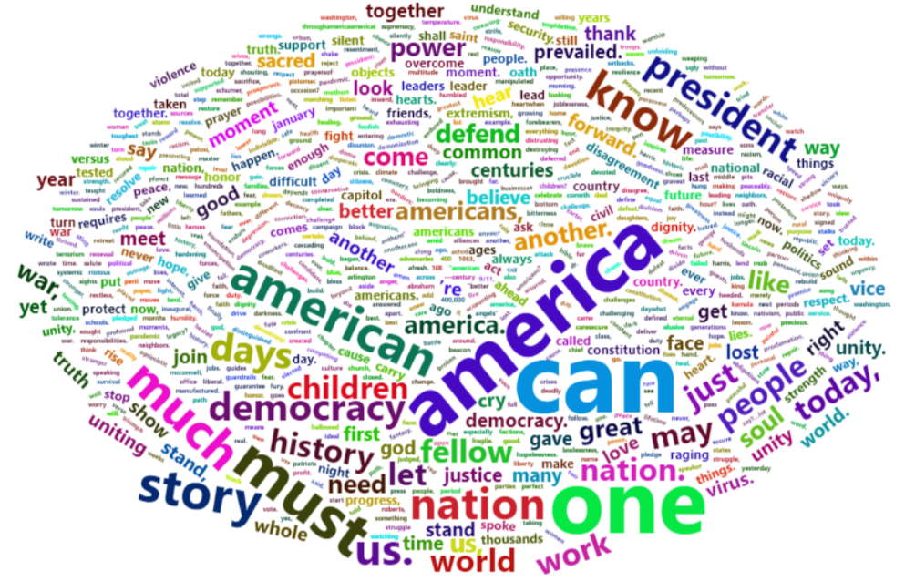

'R' 카테고리의 다른 글
| [R] 자연어 처리 - NLP (0) | 2022.02.16 |
|---|---|
| [R] 감성분석 (0) | 2022.02.16 |
| [R] 다나와 사이트 Web scrapling(selenium) (0) | 2022.02.15 |
| [R] web scraping - selenium (0) | 2022.02.10 |
| [R] web scraping - css, xpath,JSON (0) | 2022.02.10 |


